Maximum Power Transfer Theorem: Load Matching and Efficiency
A Thevenin equivalent source drives a variable load \(R_L\) | Power versus load resistance | Maximum-power condition \(R_L = R_{th}\)
Circuit Parameters
Power and Efficiency
Current Operating Point
Circuit Diagram
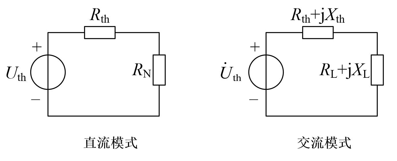
DC Maximum Power Transfer
The load receives maximum power when \(R_L\) equals \(R_{th}\):
\(P_{max} = \frac{U_{th}^2}{4 R_{th}}\)
At this point, efficiency \(\eta = 50\%\) (source internal resistance and load each consume half the power).
\(P_L = \frac{U_{th}^2 R_L}{(R_{th} + R_L)^2}\)
Matching Properties
When \(R_L\) deviates from \(R_{th}\), power decreases (parabolic shape).
As \(R_L\) increases, the power rises to a maximum and then falls.
At the maximum power point, \(R_L = R_{th}\), and the power curve reaches its peak.
Switch to AC mode to observe the complex conjugate matching condition.